
Focus on spectral sensing and optoelectronic application systems
Hyperspectral Imaging System LIBS (Laser-Induced Breakdown
Time:2025-01-14
Abstract: Accurate elemental well logs provide crucial foundational data for subsequent operations, including correctly identifying lithology, predicting the strata to be encountered during drilling, determining the stratigraphic position, selecting appropriate drilling parameters, and reducing operational risks in drilling activities.
Research on the Quantitative Multi-element Analysis Method of Wellbore Cuttings Based on LIBS Technology

1.Introduction
With the rapid development of modern society, the consumption of energy resources such as oil and natural gas has been steadily increasing, and oil and gas exploration and extraction activities have become more frequent. One of the essential tasks in the exploration and extraction of oil and gas resources is wellbore cuttings logging. In order to construct accurate wellbore logs, personnel at the drilling site must measure and record the elemental composition and content of cuttings samples collected from different well depths. Accurate elemental well logs provide critical foundational data for correctly identifying lithology, predicting the strata to be encountered, determining the position of the strata, selecting appropriate drilling parameters, and reducing drilling risks in subsequent work.
Traditional elemental analysis techniques mainly include Neutron Activation Analysis (NAA), Atomic Absorption Spectroscopy (AAS), Inductively Coupled Plasma Atomic Emission Spectroscopy (ICP-AES), and Inductively Coupled Plasma Mass Spectrometry (ICP-MS). As an emerging atomic emission spectroscopy technique, Laser-Induced Breakdown Spectroscopy (LIBS) offers several advantages, such as simple sample preparation, a compact and easy-to-miniaturize structure, the ability to simultaneously detect multiple elements, and fast analysis speeds. Due to these advantages, LIBS has been widely applied to the analysis of various substances, including food, alloys, explosives, and soil.
In this study, a quantitative analysis method for five major elements (Si, Al, Ca, Mg, and K) in rock samples will be developed for the LIBS instrument, to meet the practical needs of elemental analysis of wellbore cuttings samples at the drilling site. Finally, the detection results of LIBS will be compared with the most widely used X-Ray Fluorescence (XRF) technology for elemental analysis of wellbore cuttings to evaluate its feasibility for field application.
2.Experimental Section
2.1 Sample Preparation
A total of 163 rock samples were used in this study, which were mixed evenly using a vortex mixer. The wellbore cuttings samples were collected from different depths of the same well at a logging site in the southwestern region of China. These samples were sequentially numbered according to their increasing depth from LJ #01 to LJ #97. The target element content of this batch of samples was determined following the national standards GB/T 14506.28-2010 for chemical analysis of silicate rocks and JY/T 0569-2020 for general methods of wavelength dispersive X-ray fluorescence spectroscopy.
The rock samples used in this experiment were uniform powders, with the content of the five target elements detailed in Tables 1 and 2 in Appendix B. The samples were dried in an electric constant-temperature drying oven at 60°C for 2 hours. After drying, 1 g of each sample was weighed and pressed into circular discs with a diameter of 20 mm using an automatic pellet press under a pressure of 8 MPa for 20 seconds. Figure 1 shows a representative pressed sample.
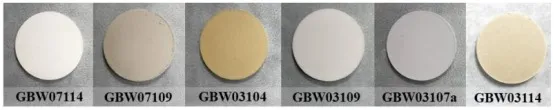
Figure 1: Representative Rock Pellet Sample
2.2 Spectral Data Acquisition
For the spectral data acquisition of the rock samples, the exposure time was set to 1 ms, and the delay time was set to 1.5 μs. Spectral data were collected from 20 randomly selected positions on the sample surface. To reduce the influence of fluctuations in the laser pulse energy on the stability of the spectral data and to further improve the signal-to-noise ratio of the spectral lines, the spectral signals were collected 4 times at each position. The average of these 4 measurements was then used as the spectral data for that specific location.
2.3 Spectral Analysis Procedure
In this study, the spectral data of 49 national standard rock samples were used as the training dataset, while the spectral data of 17 self-made supplementary samples were used as the test dataset. Based on the training dataset, quantitative analysis models for the five target elements were developed. The models' performance was evaluated using the test dataset. In the application test, 97 well logging cuttings were used as unknown samples. The LIBS instrument and the associated analysis software were used to apply the quantitative analysis models to detect the content of the five target elements. The results obtained from LIBS were then compared with the detection results from the widely used XRF technique for well logging cuttings, to evaluate the feasibility of applying this instrument in actual field conditions. Figure 2 illustrates the overall data analysis process.
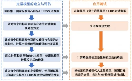
Figure 2: Schematic Diagram of the Overall Data Analysis Process
3.Results and Discussion
3.1 Spectral Data Preprocessing and Feature Line Selection
Figure 3 presents the raw spectra of representative rock pellet samples collected by the LIBS instrument. As shown in the figure, the baseline of the entire spectrum is relatively stable, and characteristic spectral lines of multiple elements such as Si, Mg, and Ca can be clearly identified. The signal-to-noise ratio (SNR) is good, indicating that the spectra collected by the instrument are sufficient for analysis needs.
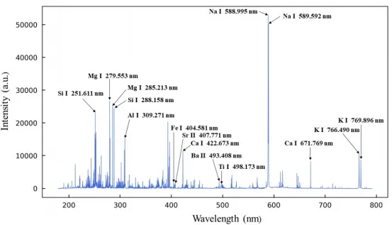
Figure 3 LIBS Spectra of Representative Rock Pellet Sample (GBW07111)
However, the stability and repeatability of LIBS spectral data can be influenced by factors such as the performance of the instrument, the homogeneity of solid powder samples, and complex matrix effects in the rock. Normalizing the spectral data can enhance its stability and repeatability. Common normalization methods include total area normalization, maximum-minimum intensity normalization, and standard normal variate (SNV) transformation.
Nevertheless, rocks contain numerous elements, and the differences in elemental concentrations across different samples can be substantial. As a result, the total intensity of the LIBS spectrum and the number of emitted spectral lines also vary between samples. For example, Figure 4 shows that the national standard samples GBW03115 and GBW07107 have similar matrices, and the concentrations of Si and Ca elements are very close. However, the Fe content differs significantly: GBW07107 contains 5.32% Fe, while GBW03115 only contains 0.60% Fe. In comparison, the LIBS spectrum of GBW07107 contains far more Fe characteristic spectral lines than other elements. In total area normalization, the intensity of all spectral lines is summed to form the denominator, which weakens the mapping relationship between the peak intensity of other elements' characteristic lines and their concentrations. While this improves data stability, it amplifies the effects of matrix interference.
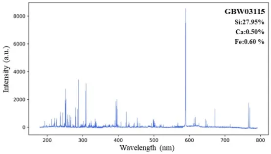
Figure 4 Comparison of LIBS Spectra for GBW03115 and GBW07107
Therefore, in this study, based on the concept of total area normalization, a partial area normalization data preprocessing method is proposed, taking into account the distribution characteristics of elements in rock samples. The method utilizes 18 characteristic spectral lines of representative elements in the rock, as listed in Table 1, for normalization:
Table 1 Characteristic Spectral Lines of Representative Elements
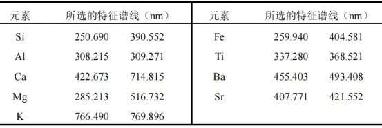
For each target element, the collected raw spectral data was compared with the NIST database, and spectral lines with strong signals and minimal interference from adjacent characteristic peaks were selected as the quantitative analysis feature peaks: 445.478 nm (Ca I), 516.732 nm (Mg I), 288.158 nm (Si I), 308.215 nm (Al I), and 769.896 nm (K I).
To determine the optimal normalization method, total area normalization, maximum-minimum intensity normalization, and partial area normalization were applied to the training set of LIBS spectral data. Calibration curves were established based on the original peak intensity, the peak intensity after preprocessing, and the corresponding element content. As shown in Figure 5, the relative standard deviation (RSD) of the original peak intensity for the selected target elements' quantitative analysis feature peaks ranged from 10% to 13.5%, indicating that the raw spectral data collected by the instrument is reliable. After normalization preprocessing, the stability and repeatability of the spectral data were further improved. The optimal normalization method for each target element was selected based on a comprehensive assessment of the spectral data stability, the overall dispersion of the rock samples, and the coefficient of determination (R²) of the calibration curves.
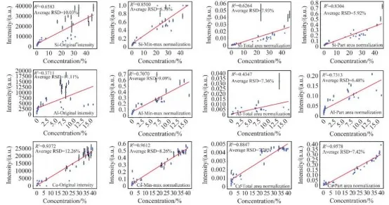

Figure 5 Calibration Curves Based on Original Peak Intensity and Peak Intensity After Different Normalization Treatments
For the element Ca, the optimal method was maximum-minimum intensity normalization. After normalization, the average RSD decreased to 8.26%, a reduction of 32.6% from the original RSD, and the R² increased from 0.9372 to 0.9612. For the element Mg, the optimal method was total area normalization. After normalization, the average RSD decreased to 8.90%, a reduction of 32.7% from the original RSD, with little change in R². For the elements Si, Al, and K, the optimal method was partial area normalization. After normalization, the average RSDs were 5.92%, 6.48%, and 7.89%, respectively, representing reductions of 41.0%, 41.7%, and 24.8% from the original RSDs. Notably, the R² values for Si and Al elements showed significant improvements, reaching 0.8304 and 0.7313, respectively.
This detailed analysis highlights the improvements in the stability and accuracy of the spectral data after applying various normalization methods, demonstrating the effectiveness of these techniques in refining LIBS-based quantitative analysis for different elements.
3.2 Establishment and Validation of Quantitative Models
After normalization using the maximum-minimum intensity method, the calibration curve for the Ca element achieved an R² value of 0.9612, indicating a strong fit. Based on this result, a quantitative model for Ca was established. However, the R² values for Mg, Si, Al, and K were not sufficiently ideal, making it challenging to directly establish accurate quantitative models for these elements. To address this, a method based on Principal Component Regression (PCR) for spectral intensity correction was proposed.
First, calibration curves for Mg, Si, Al, and K were fitted using the results from the optimal normalization methods. These curves were used to calculate the ideal peak intensities and correction coefficients for different content levels of each element. As shown in Figure 5, although the characteristic peak intensities of Al and K elements generally exhibit positive correlations with their contents, the trends vary significantly across different content ranges. To better capture the variations in peak intensity with content, a segmented fitting approach was adopted, fitting calibration curves separately for lower and higher content ranges.
The formulas for calculating ideal peak intensities and the relationships between ideal and actual peak intensities are shown in Figure 6. Using these formulas, the correction coefficients for the peak intensities can be calculated.
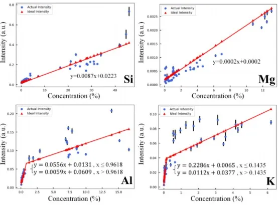
Figure 6 Ideal Peak Intensity vs. Actual Peak Intensity
The next step involves establishing a PCR (Principal Component Regression) model to calculate the peak intensity correction coefficients. Initially, PCA (Principal Component Analysis) is used to reduce the dimensionality of the spectral data and determine the appropriate number of principal components (PCs). For Mg, the total area normalization method is applied, whereas for Si, Al, and K, the partial area normalization method is used. The extracted principal components and the cumulative variance explained by these components, based on the two different normalization methods, are shown in Figure 7.
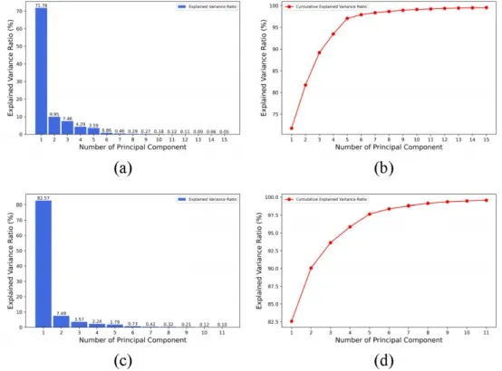
Figure 7 Analysis of Principal Components and Cumulative Variance Explained
(a) Variance Explained by the First 11 Principal Components after Partial Area Normalization
(b) Cumulative Variance Explained by the First 11 Principal Components after Partial Area Normalization
(c) Variance Explained by the First 15 Principal Components after Total Area Normalization
(d) Cumulative Variance Explained by the First 15 Principal Components after Total Area Normalization
As shown in the figures, these principal components represent the majority of the information contained in the spectral data of the training set. Using these principal components as independent variables and the correction coefficients as dependent variables, PCR (Principal Component Regression) models were established to calculate the correction coefficients.
By using the PCR models, the correction coefficients for peak intensity are calculated and then multiplied by the normalized peak intensity to obtain the corrected peak intensity. Based on this, quantitative analysis models for Mg, Si, Al, and K elements were developed. The final quantitative analysis models for all five target elements are shown in Figure 8.
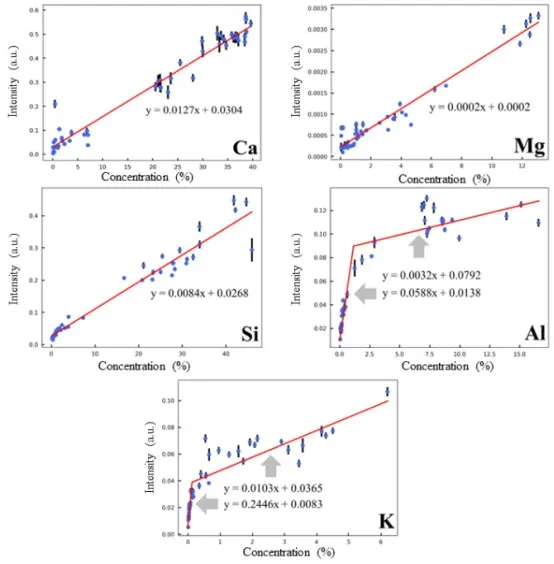
Figure 8 Quantitative Models for Target Elements
The spectral data of 17 supplementary samples in the test set were used to evaluate the accuracy of the quantitative model predictions. The predicted results for the content of the five target elements are shown in Figure 9. Overall, the model effectively predicts the content of the target elements, with R² values of 0.9843, 0.9901, 0.9745, and 0.9411 for Ca, Mg, Si, and Al elements respectively. However, the prediction performance for the K element is less satisfactory, with an R² of only 0.8114. This is attributed to the self-absorption effect that occurs at higher K element concentrations, which negatively impacts the accuracy of the quantitative model.
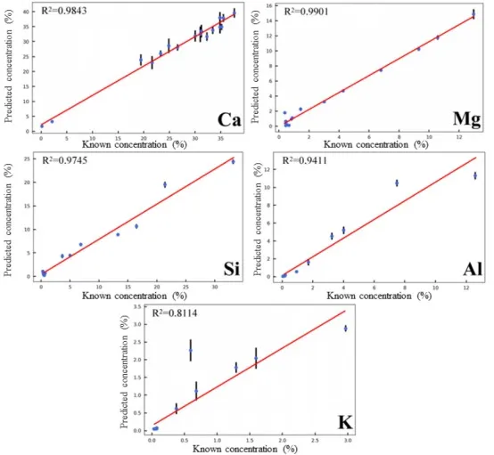
Figure 9 Prediction Performance of the Quantitative Model for Target Element Content in the Test Set
3.3 Application Testing
The established quantitative models were integrated into the LIBS instrument used, and an application test was conducted using rock cuttings samples collected from a logging site to verify the feasibility of this instrument for real-time, on-site cuttings analysis. The detection results of the five target elements using the LIBS instrument were compared with those obtained using a laboratory XRF instrument, as shown in Figure 10. The overall trends in the detection results of Ca, Mg, Si, Al, and K elements were consistent between the two instruments.
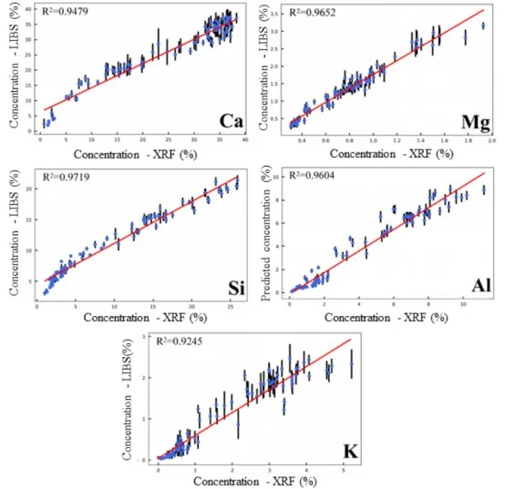
Figure 10 Detection Results of Five Element Contents in Rock Cuttings Samples
Based on the results of the application tests, trend graphs of the target element content variations were plotted, as shown in Figure 11. In the figure, the red curve represents the detection results of the LIBS instrument, and the blue curve represents the detection results of the XRF instrument. The overall trend of the two curves is consistent.
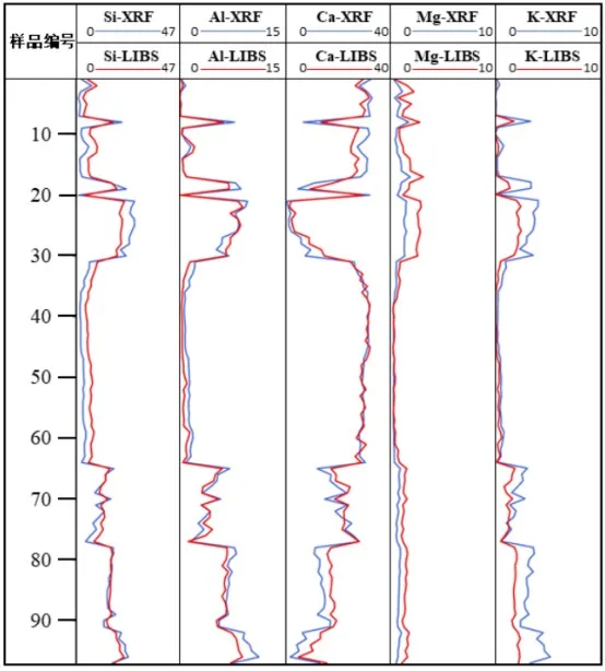 Figure 11 Trend Graph of Five Element Contents in Rock Cuttings Samples
Based on the variations in the LIBS curve, the lithology of the rock cuttings samples and the changes in the stratigraphic layers can be analyzed:
For rock cuttings samples LJ #22 to LJ #30, the detected Ca element content is mostly below 10%, Al element content is around 7%, and Si element content is around 20%. The element distribution in these samples is characteristic of clay rocks such as mudstone or shale.
For rock cuttings samples LJ #31 to LJ #64, the detected Ca element content is generally above 30%, Mg element content is below 1%, and Si element content is below 10%. The element distribution in these samples is characteristic of limestone.
From these results, it can be concluded that the lithology and the stratigraphic layers of the rock cuttings samples LJ #22 to LJ #30 are different from those of LJ #31 to LJ #64. A significant change in lithology and stratigraphy occurs starting from the location of LJ #31. This conclusion aligns with the actual conditions observed at the drilling site, indicating that the LIBS instrument integrated with the quantitative model can effectively analyze the elements in the logging rock cuttings samples, demonstrating the instrument's application potential in oil and gas exploration and extraction.
However, the study in this chapter is limited to a few elements, and the LIBS detection results for K elements are generally lower than those of XRF, while the Mg element detection results are generally higher than those of XRF. This indicates that the accuracy of the detection results needs further improvement. Therefore, future research should aim to expand the variety of elements analyzed, establish more comprehensive quantitative analysis models, and develop more accurate quantitative analysis methods.
4、Conclusion
This chapter proposes a partial area normalization data preprocessing method for rock samples and a peak intensity correction method based on Principal Component Regression (PCR). Quantitative analysis models for five elements (Ca, Mg, Si, Al, and K) were established. Using the LIBS instrument, the contents of these five elements in actual logging rock cuttings samples were detected and compared with the results obtained from laboratory XRF instruments.
The content of target elements in actual logging rock cuttings samples was measured and compared with the widely used XRF technology in the field of elemental logging. Based on the results of the two techniques, a trend graph of elemental content variations was plotted. From the graph, the lithology of the cuttings and the stratigraphic changes can be analyzed. The analysis results are consistent with the actual conditions at the drilling site.
These findings demonstrate that the portable desktop LIBS instrument, combined with the quantitative analysis methods developed in this chapter, can effectively perform real-time analysis of logging rock cuttings samples. This shows great potential for application in the field of oil and gas exploration and development.
Given that plant traits determined by genes can also be influenced by surrounding environmental changes, including soil characteristics, future research will continue to explore soil element composition based on LIBS technology. The goal is to describe the variations and correlations of element compositions in various plant tissue types and soil sample types.
Recommendation:
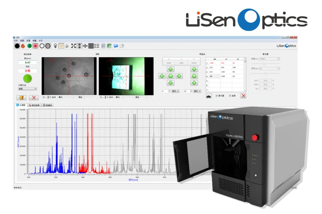
Integrated LIBS Laser-Induced Breakdown Spectrometer iSpecLIBS-SCI800
The iSpecLIBS-SCI800 is an integrated system primarily composed of a laser, a high-resolution spectrometer, LIBS optical collection probe, XYZ sample window, and trigger delay controller. Due to its integrated design, the system is highly flexible and expandable, making it an ideal solution for research applications, LIBS optical experiments, and optical application centers. Users can easily and flexibly configure the laser and spectrometer based on their specific requirements.
Abstract: Accurate elemental well logs provide crucial foundational data for subsequent operations, including correctly identifying lithology, predicting the strata to be encountered during drilling, determining the stratigraphic position, selecting appropriate drilling parameters, and reducing operational risks in drilling activities.
Research on the Quantitative Multi-element Analysis Method of Wellbore Cuttings Based on LIBS Technology
1.Introduction
With the rapid development of modern society, the consumption of energy resources such as oil and natural gas has been steadily increasing, and oil and gas exploration and extraction activities have become more frequent. One of the essential tasks in the exploration and extraction of oil and gas resources is wellbore cuttings logging. In order to construct accurate wellbore logs, personnel at the drilling site must measure and record the elemental composition and content of cuttings samples collected from different well depths. Accurate elemental well logs provide critical foundational data for correctly identifying lithology, predicting the strata to be encountered, determining the position of the strata, selecting appropriate drilling parameters, and reducing drilling risks in subsequent work.
Traditional elemental analysis techniques mainly include Neutron Activation Analysis (NAA), Atomic Absorption Spectroscopy (AAS), Inductively Coupled Plasma Atomic Emission Spectroscopy (ICP-AES), and Inductively Coupled Plasma Mass Spectrometry (ICP-MS). As an emerging atomic emission spectroscopy technique, Laser-Induced Breakdown Spectroscopy (LIBS) offers several advantages, such as simple sample preparation, a compact and easy-to-miniaturize structure, the ability to simultaneously detect multiple elements, and fast analysis speeds. Due to these advantages, LIBS has been widely applied to the analysis of various substances, including food, alloys, explosives, and soil.
In this study, a quantitative analysis method for five major elements (Si, Al, Ca, Mg, and K) in rock samples will be developed for the LIBS instrument, to meet the practical needs of elemental analysis of wellbore cuttings samples at the drilling site. Finally, the detection results of LIBS will be compared with the most widely used X-Ray Fluorescence (XRF) technology for elemental analysis of wellbore cuttings to evaluate its feasibility for field application.
2.Experimental Section
2.1 Sample Preparation
A total of 163 rock samples were used in this study, which were mixed evenly using a vortex mixer. The wellbore cuttings samples were collected from different depths of the same well at a logging site in the southwestern region of China. These samples were sequentially numbered according to their increasing depth from LJ #01 to LJ #97. The target element content of this batch of samples was determined following the national standards GB/T 14506.28-2010 for chemical analysis of silicate rocks and JY/T 0569-2020 for general methods of wavelength dispersive X-ray fluorescence spectroscopy.
The rock samples used in this experiment were uniform powders, with the content of the five target elements detailed in Tables 1 and 2 in Appendix B. The samples were dried in an electric constant-temperature drying oven at 60°C for 2 hours. After drying, 1 g of each sample was weighed and pressed into circular discs with a diameter of 20 mm using an automatic pellet press under a pressure of 8 MPa for 20 seconds. Figure 1 shows a representative pressed sample.
Figure 1: Representative Rock Pellet Sample
2.2 Spectral Data Acquisition
For the spectral data acquisition of the rock samples, the exposure time was set to 1 ms, and the delay time was set to 1.5 μs. Spectral data were collected from 20 randomly selected positions on the sample surface. To reduce the influence of fluctuations in the laser pulse energy on the stability of the spectral data and to further improve the signal-to-noise ratio of the spectral lines, the spectral signals were collected 4 times at each position. The average of these 4 measurements was then used as the spectral data for that specific location.
2.3 Spectral Analysis Procedure
In this study, the spectral data of 49 national standard rock samples were used as the training dataset, while the spectral data of 17 self-made supplementary samples were used as the test dataset. Based on the training dataset, quantitative analysis models for the five target elements were developed. The models' performance was evaluated using the test dataset. In the application test, 97 well logging cuttings were used as unknown samples. The LIBS instrument and the associated analysis software were used to apply the quantitative analysis models to detect the content of the five target elements. The results obtained from LIBS were then compared with the detection results from the widely used XRF technique for well logging cuttings, to evaluate the feasibility of applying this instrument in actual field conditions. Figure 2 illustrates the overall data analysis process.
Figure 2: Schematic Diagram of the Overall Data Analysis Process
3.Results and Discussion
3.1 Spectral Data Preprocessing and Feature Line Selection
Figure 3 presents the raw spectra of representative rock pellet samples collected by the LIBS instrument. As shown in the figure, the baseline of the entire spectrum is relatively stable, and characteristic spectral lines of multiple elements such as Si, Mg, and Ca can be clearly identified. The signal-to-noise ratio (SNR) is good, indicating that the spectra collected by the instrument are sufficient for analysis needs.
Figure 3 LIBS Spectra of Representative Rock Pellet Sample (GBW07111)
However, the stability and repeatability of LIBS spectral data can be influenced by factors such as the performance of the instrument, the homogeneity of solid powder samples, and complex matrix effects in the rock. Normalizing the spectral data can enhance its stability and repeatability. Common normalization methods include total area normalization, maximum-minimum intensity normalization, and standard normal variate (SNV) transformation.
Nevertheless, rocks contain numerous elements, and the differences in elemental concentrations across different samples can be substantial. As a result, the total intensity of the LIBS spectrum and the number of emitted spectral lines also vary between samples. For example, Figure 4 shows that the national standard samples GBW03115 and GBW07107 have similar matrices, and the concentrations of Si and Ca elements are very close. However, the Fe content differs significantly: GBW07107 contains 5.32% Fe, while GBW03115 only contains 0.60% Fe. In comparison, the LIBS spectrum of GBW07107 contains far more Fe characteristic spectral lines than other elements. In total area normalization, the intensity of all spectral lines is summed to form the denominator, which weakens the mapping relationship between the peak intensity of other elements' characteristic lines and their concentrations. While this improves data stability, it amplifies the effects of matrix interference.
Figure 4 Comparison of LIBS Spectra for GBW03115 and GBW07107
Therefore, in this study, based on the concept of total area normalization, a partial area normalization data preprocessing method is proposed, taking into account the distribution characteristics of elements in rock samples. The method utilizes 18 characteristic spectral lines of representative elements in the rock, as listed in Table 1, for normalization:
Table 1 Characteristic Spectral Lines of Representative Elements
For each target element, the collected raw spectral data was compared with the NIST database, and spectral lines with strong signals and minimal interference from adjacent characteristic peaks were selected as the quantitative analysis feature peaks: 445.478 nm (Ca I), 516.732 nm (Mg I), 288.158 nm (Si I), 308.215 nm (Al I), and 769.896 nm (K I).
To determine the optimal normalization method, total area normalization, maximum-minimum intensity normalization, and partial area normalization were applied to the training set of LIBS spectral data. Calibration curves were established based on the original peak intensity, the peak intensity after preprocessing, and the corresponding element content. As shown in Figure 5, the relative standard deviation (RSD) of the original peak intensity for the selected target elements' quantitative analysis feature peaks ranged from 10% to 13.5%, indicating that the raw spectral data collected by the instrument is reliable. After normalization preprocessing, the stability and repeatability of the spectral data were further improved. The optimal normalization method for each target element was selected based on a comprehensive assessment of the spectral data stability, the overall dispersion of the rock samples, and the coefficient of determination (R²) of the calibration curves.
Figure 5 Calibration Curves Based on Original Peak Intensity and Peak Intensity After Different Normalization Treatments
For the element Ca, the optimal method was maximum-minimum intensity normalization. After normalization, the average RSD decreased to 8.26%, a reduction of 32.6% from the original RSD, and the R² increased from 0.9372 to 0.9612. For the element Mg, the optimal method was total area normalization. After normalization, the average RSD decreased to 8.90%, a reduction of 32.7% from the original RSD, with little change in R². For the elements Si, Al, and K, the optimal method was partial area normalization. After normalization, the average RSDs were 5.92%, 6.48%, and 7.89%, respectively, representing reductions of 41.0%, 41.7%, and 24.8% from the original RSDs. Notably, the R² values for Si and Al elements showed significant improvements, reaching 0.8304 and 0.7313, respectively.
This detailed analysis highlights the improvements in the stability and accuracy of the spectral data after applying various normalization methods, demonstrating the effectiveness of these techniques in refining LIBS-based quantitative analysis for different elements.
3.2 Establishment and Validation of Quantitative Models
After normalization using the maximum-minimum intensity method, the calibration curve for the Ca element achieved an R² value of 0.9612, indicating a strong fit. Based on this result, a quantitative model for Ca was established. However, the R² values for Mg, Si, Al, and K were not sufficiently ideal, making it challenging to directly establish accurate quantitative models for these elements. To address this, a method based on Principal Component Regression (PCR) for spectral intensity correction was proposed.
First, calibration curves for Mg, Si, Al, and K were fitted using the results from the optimal normalization methods. These curves were used to calculate the ideal peak intensities and correction coefficients for different content levels of each element. As shown in Figure 5, although the characteristic peak intensities of Al and K elements generally exhibit positive correlations with their contents, the trends vary significantly across different content ranges. To better capture the variations in peak intensity with content, a segmented fitting approach was adopted, fitting calibration curves separately for lower and higher content ranges.
The formulas for calculating ideal peak intensities and the relationships between ideal and actual peak intensities are shown in Figure 6. Using these formulas, the correction coefficients for the peak intensities can be calculated.
Figure 6 Ideal Peak Intensity vs. Actual Peak Intensity
The next step involves establishing a PCR (Principal Component Regression) model to calculate the peak intensity correction coefficients. Initially, PCA (Principal Component Analysis) is used to reduce the dimensionality of the spectral data and determine the appropriate number of principal components (PCs). For Mg, the total area normalization method is applied, whereas for Si, Al, and K, the partial area normalization method is used. The extracted principal components and the cumulative variance explained by these components, based on the two different normalization methods, are shown in Figure 7.
Figure 7 Analysis of Principal Components and Cumulative Variance Explained
(a) Variance Explained by the First 11 Principal Components after Partial Area Normalization
(b) Cumulative Variance Explained by the First 11 Principal Components after Partial Area Normalization
(c) Variance Explained by the First 15 Principal Components after Total Area Normalization
(d) Cumulative Variance Explained by the First 15 Principal Components after Total Area Normalization
As shown in the figures, these principal components represent the majority of the information contained in the spectral data of the training set. Using these principal components as independent variables and the correction coefficients as dependent variables, PCR (Principal Component Regression) models were established to calculate the correction coefficients.
By using the PCR models, the correction coefficients for peak intensity are calculated and then multiplied by the normalized peak intensity to obtain the corrected peak intensity. Based on this, quantitative analysis models for Mg, Si, Al, and K elements were developed. The final quantitative analysis models for all five target elements are shown in Figure 8.
Figure 8 Quantitative Models for Target Elements
The spectral data of 17 supplementary samples in the test set were used to evaluate the accuracy of the quantitative model predictions. The predicted results for the content of the five target elements are shown in Figure 9. Overall, the model effectively predicts the content of the target elements, with R² values of 0.9843, 0.9901, 0.9745, and 0.9411 for Ca, Mg, Si, and Al elements respectively. However, the prediction performance for the K element is less satisfactory, with an R² of only 0.8114. This is attributed to the self-absorption effect that occurs at higher K element concentrations, which negatively impacts the accuracy of the quantitative model.
Figure 9 Prediction Performance of the Quantitative Model for Target Element Content in the Test Set
3.3 Application Testing
The established quantitative models were integrated into the LIBS instrument used, and an application test was conducted using rock cuttings samples collected from a logging site to verify the feasibility of this instrument for real-time, on-site cuttings analysis. The detection results of the five target elements using the LIBS instrument were compared with those obtained using a laboratory XRF instrument, as shown in Figure 10. The overall trends in the detection results of Ca, Mg, Si, Al, and K elements were consistent between the two instruments.
Figure 10 Detection Results of Five Element Contents in Rock Cuttings Samples
Based on the results of the application tests, trend graphs of the target element content variations were plotted, as shown in Figure 11. In the figure, the red curve represents the detection results of the LIBS instrument, and the blue curve represents the detection results of the XRF instrument. The overall trend of the two curves is consistent.
Figure 11 Trend Graph of Five Element Contents in Rock Cuttings Samples
Based on the variations in the LIBS curve, the lithology of the rock cuttings samples and the changes in the stratigraphic layers can be analyzed:
For rock cuttings samples LJ #22 to LJ #30, the detected Ca element content is mostly below 10%, Al element content is around 7%, and Si element content is around 20%. The element distribution in these samples is characteristic of clay rocks such as mudstone or shale.
For rock cuttings samples LJ #31 to LJ #64, the detected Ca element content is generally above 30%, Mg element content is below 1%, and Si element content is below 10%. The element distribution in these samples is characteristic of limestone.
From these results, it can be concluded that the lithology and the stratigraphic layers of the rock cuttings samples LJ #22 to LJ #30 are different from those of LJ #31 to LJ #64. A significant change in lithology and stratigraphy occurs starting from the location of LJ #31. This conclusion aligns with the actual conditions observed at the drilling site, indicating that the LIBS instrument integrated with the quantitative model can effectively analyze the elements in the logging rock cuttings samples, demonstrating the instrument's application potential in oil and gas exploration and extraction.
However, the study in this chapter is limited to a few elements, and the LIBS detection results for K elements are generally lower than those of XRF, while the Mg element detection results are generally higher than those of XRF. This indicates that the accuracy of the detection results needs further improvement. Therefore, future research should aim to expand the variety of elements analyzed, establish more comprehensive quantitative analysis models, and develop more accurate quantitative analysis methods.
4、Conclusion
This chapter proposes a partial area normalization data preprocessing method for rock samples and a peak intensity correction method based on Principal Component Regression (PCR). Quantitative analysis models for five elements (Ca, Mg, Si, Al, and K) were established. Using the LIBS instrument, the contents of these five elements in actual logging rock cuttings samples were detected and compared with the results obtained from laboratory XRF instruments.
The content of target elements in actual logging rock cuttings samples was measured and compared with the widely used XRF technology in the field of elemental logging. Based on the results of the two techniques, a trend graph of elemental content variations was plotted. From the graph, the lithology of the cuttings and the stratigraphic changes can be analyzed. The analysis results are consistent with the actual conditions at the drilling site.
These findings demonstrate that the portable desktop LIBS instrument, combined with the quantitative analysis methods developed in this chapter, can effectively perform real-time analysis of logging rock cuttings samples. This shows great potential for application in the field of oil and gas exploration and development.
Given that plant traits determined by genes can also be influenced by surrounding environmental changes, including soil characteristics, future research will continue to explore soil element composition based on LIBS technology. The goal is to describe the variations and correlations of element compositions in various plant tissue types and soil sample types.
Recommendation:
Integrated LIBS Laser-Induced Breakdown Spectrometer iSpecLIBS-SCI800
The iSpecLIBS-SCI800 is an integrated system primarily composed of a laser, a high-resolution spectrometer, LIBS optical collection probe, XYZ sample window, and trigger delay controller. Due to its integrated design, the system is highly flexible and expandable, making it an ideal solution for research applications, LIBS optical experiments, and optical application centers. Users can easily and flexibly configure the laser and spectrometer based on their specific requirements.
Previous: No data
PRODUCTS
Copyright © 2025 Lisen Optics (Shenzhen) Co., Ltd.